- Overview
- Estimation model
- Working with Regression analysis
- Forecast
- Report
- Calculating regression with formulas
- Examples
- Questions
Overview
Example of general use of Regression analysis:
The Regression analysis implements a multiple linear regression model. The analysis aims to model the relationship between a dependent series and one or more explanatory series. Several models can be specified within one instance of the analysis. The output consists of the coefficients of the linear model, the predicted series, and several statistical indicators. If there is sufficient data after the end of the estimation sample range, forecasts can be calculated.
Estimation model
The Regression can only calculate static linear regression model. Analysis attempts to find the linear combination of a number of explanatory series that best describes a dependent series.
 ⇒
⇒ 
The analysis uses the following Ordinary Least Squares (OLS) model:
| y | dependent series |
| x_i | explanatory series |
| α | intercept |
| β | slope (coefficient, beta) |
| ϵ | sum of the squared residuals (sum of squared errors) |
If the option No intercept is selected in analysis, then the constant α is not included in the model.
The parameters α and β are estimated by minimizing the sum of the squared residuals ϵ. The output from the analysis will include the predicted series calculated using the estimated parameters.
The automatic estimation sample range will be the largest range where there is data for all series. You can specify a smaller range if you like to limit the data to be used in the estimation.
Working with Regression analysis
Settings

Regression models
You can define one or more regression models. Each model has separate settings. When a new model is created, the settings of the current model are duplicated. Models can be renamed and deleted.
Output dependent series
Select this option to include the dependent series in the output.
Output explanatory series
Select this option to include the explanatory series in the output.
Estimation sample range
Specify the limits of the estimation sample range. The default range will be the largest range where there is data for all the series.
No intercept
When this option is selected, the constant α is omitted from the model and it will be defined as:
Residuals
When this option is selected a series containing the residuals will be included in the output.
Residuals for forecasts
If this option is selected, the series of residuals will also contain residuals for the forecasted values. Such residuals can only be calculated when forecasts are calculated and there is an overlap between the forecasts and the dependent series.
Uncertainty band
By selecting the option Uncertainty band, two additional time series will be calculated. These time series form a band around the predicted values by adding and subtracting a number of standard deviations. The standard deviations are based on Standard error of regression which is calculated as 'the square root of the sum of squared forecast residuals divided by the number of residuals', as described in the section Report.
Calculate forecasts
Forecasts will be calculated only if this option is selected and there is sufficient data, as explained in the section Forecast.
End point
You can limit how far into the future that forecasts will be calculated. If not specified, forecasts will be calculated as far as possible.
Allow dynamic forecast
Allow the use of predicted values of the dependent series when calculating forecasts. See more under Dynamic Forecast.
Confidence band
By selecting the option Confidence band, two additional series will be calculated. These time series form a confidence band around the forecasted values. The band is calculated so that the forecast is within the band with the specified probability assuming that the forecast values are t-distributed.
Series settings

Include
Select if you want to include this series in the model.
Is dependent
Select which series is the dependent series. This must be specified.
Diff
By selecting Diff, the first order differences of the series will be calculated. The result will then be converted back to levels. First order of differences means that the series is transformed to 'Change over value (one observation)' while expressing the result in levels. If you tick that option, the result will output the coefficients for intercept and diff(x1) rather than intercept and x1.
Diff->legacy
Calculate the predicted series by adding diffs to the dependent series (it was a default option for Macrobond version 1.26 and lower).
This setting does not affect the model itself. It only influences the step after the calculation of the model when the levels are calculated from the differences.
Diff->agg
Calculate the predicted series by aggregating the predicted differentials.
Lag to/from and Lag range
Here you specify the lags you would like to include for a specific series. When lagging a series, the values are delayed in time and the series stretches further into the future.
If you for example set 'Lag from' to 0 and 'Lag to' to 2 three series will be included, one series with no lag, one with a lag of 1 and one series with 2 lags. This will automatically change the lag range to '0 to 2'. You may specify the desired lags using 'Lag to/from' or 'Lag range', the result will be the same. If you set Lag range to a single digit or set Lag to and 'Lag from' to the same value, a single lagged series will be included.
When lags are specified for the dependent series, the lagged series will be used as explanatory series in the model. The dependent series will always be without lag.
How to create simple regression model?
- Check boxes for 'Output the dependent series' and 'Output the explanatory series'.
- Check 'Include' for at least two series and mark one as 'Is dependent'.
- Add Scatter chart. Go there and open Graph layout (Ctrl+L).
- Pair series to generate a regression line. Make sure to set the right order of the series in Graph layout window (Note that when series is lagged there won't be a straight line as outcome.):
a) Pair #1: the explanatory and the dependent series
b) Pair #2: the explanatory and the predicted series

Line A Line B series 1 series 1 series 2 series 2 [predicted] - Click on one of the lines, go to Presentation properties > Appearance, change Graph style to Custom. Then set Line to None and select Marker style.
How to add best fit line through different series' last values?
With formula output only last value from each series. Lag each value and glue them together with Cross section creating fake time series which can be fed to Regression analysis. See the file with explanation under Best fit line for last values of group of series with and WITHOUT Regression analysis.
Common errors
Too few time series in graph
- Check if you have added Category scatter chart - use Scatter chart instead.
- In left panel you should see at least 3 series in the output. Check if you have enabled 'Output dependent series' and 'Output explanatory series' at the top in Regression analysis.
- Check if you have two pairs of series in Graph layout. If not, see how to pair them under How to create simple regression model?.
Degree of freedom is too low
You cannot fit the regression coefficients if there are no degrees of freedom. The degrees of freedom is the number of observations - number of parameters that we are estimating. The number of estimated parameters includes the intercept.
The number of observations must thus be larger than the number of independent (explanatory) series.
This might be caused for example by changing document's frequency to lower (i.e., from Monthly to Annual) or series used have not enough overlapping observations.
Forecast
How it works?

When there are data for all the explanatory series beyond the estimation sample, we can use the estimated parameters to calculate forecasts. This is done by checking the option 'Calculate forecast'. If no end point is specified, the analysis will calculate as many forecasted values as possible. You can specify an end point if you want to limit the length of the forecast. End point refers to 'up to, but not including'.
Forecast can't go further than the longest common part of explanatory series.
See Regression - how forecast is calculated file.
Dynamic forecast
Dynamic forecasting uses the data generated by the model as inputs to extend the forecast horizon. In this setup, the dependent series serves as an explanatory variable through its lag.
 ⇒
⇒ 
Standard Regression analysis ⇒ How dynamic forecast is created
Enabling the Dynamic forecast option helps in two ways:
- Extending the forecast horizon when external variables have longer lags than the dependent variable.
In static forecasting, the horizon is limited by the shortest lag among both dependent and the explanatory variables. With dynamic forecasting enabled, the model fills in the missing lagged dependent values using previously predicted data. This allows the forecast to extend further, up to the point common for all external explanatory variables. - Producing an infinite forecast.
If no external explanatory variables are used, and the model is driven solely by lagged values of the dependent variable, the forecast can be projected far ahead. In this case, the model keeps feeding itself with its own lagged forecasts. To achieve that:- add second Model under Regression models;
- include only main series, mark it as dependent;
- set at least 1 lag to it;
- check box for 'Allow dynamic forecast' under Forecast panel;
- specify an 'End point' for the forecast because there is no way for the application to know when to stop.
End date
The estimation sample range in the Regression analysis is used for calculating the regression parameters. This range is not used for calculating the forecast. To limit the data used in all cases we recommend setting the data range on the Series list.
Report
Overview
The Regression analysis automatically generates a report, which includes variety of statistical information.

Calculation range
The calculation range used for the analysis.
Observations
The number of observations used in the analysis. This includes all observations in the calculation range where there are values for all series.
Degrees of freedom
The number of observations minus the number of explanatory series and minus one for the constant parameter.
R2
Compares the variance of the estimation with the total variance. The better the result fits the data compared to a simple average, the closer this value is to 1.
In the ordinary case when an intercept term is included, this value is calculated as the square of the correlation between the dependent series and the estimate. In this case R2 will always be between 0 and 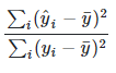
If the option "No intercept" has been selected, R2 is calculated in a different way since the dependent and estimated series can now have different mean values.

Please note that R2 for models that allow an intercept term cannot be compared with models that do not allow intercept. Typically, R2 for models that do not allow intercept, will be higher than the corresponding model with intercept, but that does not mean that it is a better fit.
Adjusted R2
To overcome the issue with R2 that it will always be higher when you add more variables to your model, you often look at the adjusted R2 that is calculated in the following way:
1-(1-R2)*(n-1)/(df-1)
Where n is the length of the series and df is the degrees of freedom.
F
The F-ratio is the ratio of the explained variability and the unexplained variability each divided by the corresponding degrees of freedom. In general, a larger F, indicates a more useful model.
P-value (F)
The p-value is the probability of obtaining a value of F that is at least as extreme as the one that was actually observed if the true values of all the coefficients are zero.
Sum of squared errors
The sum of the square of the residuals.
Standard error of regression
The square root of the sum of squared errors divided by the degrees of freedom. This is an estimate of the standard deviation of residuals.
Standard error of forecasts
The square root of the sum of squared forecast residuals divided by the number of residuals.
Durbin-Watson
The Durbin-Watson is a test statistic used to detect the presence of autocorrelation in the residuals. The value is in the range 0-4. A value close to 2 means that there is little auto correlation. Values from 0 to less than 2 point to positive autocorrelation and values from 2 to 4 means negative autocorrelation. The result from this test is not useful if any dependent series is included with several lags or if no intercept is included in the model.
For more information about this see Investopedia.
Information criteria
The information criteria are measures of the expected information loss. A lower value means that more information is captured. This can be used to compare models when the same data is used in the models.
AIC
Akaike's information criterion.
HQ
Hannan and Quinn's information criterion
Schwarz
Schwarz criterion also known as Bayesian information criterion
Coefficient
The estimated parameters
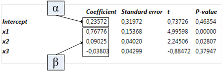
Standard error
The standard error of the estimated parameters
t
The estimated coefficient divided by the standard error
P-value
The p-value is the probability of obtaining a value of t that is at least as extreme as the one that was actually observed if the true value of the coefficient is zero
How to output coefficients?
This analysis doesn’t produce as output the coefficients from the models. In main application they are only available in the 'Regression report'.
You can access them through Excel add-in, to do this:
- Right click on Series list and select 'Copy your series as Excel data set'. Paste it to Excel.
- Right click on red object, go to Edit. In new window as Select output, choose Regression and in next field Category series.
You can also calculate them separately in main application - see Calculating regression with formulas.
Errors
Sometimes Model cannot be calculated and instead you will see error message indicating what is preventing calculation.
Calculation range end date is before start date
One (or more) series is too short. Check them on Time table before Regression analysis and exclude it from the calculation.
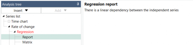
There is a linear dependency between the independent series
This means the equation system cannot be solved due to arbitrary values can be assigned to one or more of the constants in the equation and residuals can't be calculated.
Usually it appears when you turn frequency of series from lower (i.e., Annual) to higher (i.e., Monthly) thus those series have repeated values for an entire period. As a solution go to Conversion settings tab > To higher... and select there 'Cubic interpolation'. Some further manipulation might be needed (i.e., deleting lags for some series) but it depends on composition of your model.
Degrees of freedom is too low
You cannot fit the regression coefficients if there are no degrees of freedom. The degrees of freedom is the number of observations - number of parameters that we are estimating. The number of estimated parameters includes the intercept.
The number of observations must thus be larger than the number of independent (explanatory) series.
This might be caused for example by changing document's frequency to lower (i.e., from Monthly to Annual) or series used have not enough overlapping observations.
Calculating regression with formulas
To calculate α, β and R2 use:
Intercept(series1, series2)
Slope(series1, series2)
Pow(Correlation(series1, series2), 2)
where series1 is the dependent series and series2 is the explanatory series. If you get different values than from analysis check 'Estimation sample range' - it has to be calculated on identical time range. To avoid adding Cut() formula everywhere you can set data range on Series list.
Formulas above calculate the regression between two series, but if in Regression analysis are more series these won't be comparable models - you will get different outcomes.
Showing regression formula on chart
You can generate the y=ax+b formula with these formulas in Text box using Dynamic text:
y = {s s1.Value}*x + {s s2.Value}
where s1 and s2 indicate α and β series. Note that in your chart those series could be s31 and s43 or any other number. To check this double-click on text area (i.e., Text box) and see Dynamic properties panel on the right side:
Examples
In the Regression analysis, we first defined the variables of the model, by:
- Marking the Industrial Production as dependent variable
- Specifying the lags for the explanatory series (these numbers are based on the Correlation analysis).
- Defining the output, we want to have in the chart: dependent series & residuals
We also decided to calculate forecasts. This is possible as all explanatory variables have been lagged, meaning we can calculate forecasts for the shortest number of lags defined, here 2 months.
In the Regression analysis, we checked as output both the dependent and explanatory variables. Both series, as well as the predicted series, will be needed in the Scatter Chart to show one week change in both in indices.
Regression model for three series with expanding window and outputted coefficients.
In the Regression analysis thanks to formulas you can display equation on chart.
An example showing how forecast with lagged series work.
An example showing dynamic forecast in use.
Estimation of the Phillips curve based on the observations with fit line created through Regression.
Best fit line for last values of group of series with and WITHOUT Regression analysis
See how to prepare series to show best fit line for last values of group of series in Regression analysis and also how to do this without Regression at all - only through calculations.
Questions
- Can I add non-linear regression?
- From where it is taking its residual?
- How to add dummy variable?
- How to do a logarithmic regression?
- How to do a regression against time (on one series)?
- Why model's values are different than the ones coming from a same model but rolling?
Can I add non-linear regression?
Generally no, but in Examples you can find Philips curve built with Regression.
From where it is taking its residual?
The residual stems from the difference between the predicted model and its main series.
How to add dummy variable?
You can create binary series (0/1 series) using conditions in the formula language. These formulas need to be applied before the regression analysis. In Regression please add such series as explanatory.
For example:
quarter()=1|quarter()=3
Returns 1 if the observation is Q1 or Q3, 0 otherwise.
quarter()=1 & year()=2020|quarter()=3 & year()=2020
Returns 1 if the observation is Q1 or Q3 for year 2020, 0 otherwise. Each quarter must have '& year()=2020' parameter, otherwise it will point to quarters in each year.
DayOfWeek()=5
Returns 1 if the observation is a Friday, 0 otherwise.
Counter()=EndOfYear()
Returns 1 if the observation is the last one in a year, 0 otherwise.
Counter()=Date(2020, 4, 1)
Returns 1 if the observation is a 1st April 2020, 0 otherwise.
Cop(usgdp, yearlength())<0
Returns 1 if the US GDP y/y growth rate is negative, 0 otherwise.
For more information see: Built-in formula functions
How to do a logarithmic regression?
You can calculate it with formulas but express the explanatory variable as Log(series).
For more information see: Built-in formula functions
How to do a regression against time (on one series)?
To perform linear regression on one time series (where the independent variable is time) use Counter() on Series list and perform Regression analysis.
For more information see: Built-in formula functions
Why model's values are different than the ones coming from a same model but rolling?
The differences stems from different time ranges being taken into calculation because of:
- Mon-Sun daily series vs Mon-Fri daily series
- what Macrobond takes into account when calculating a sample range
To ensure that you are looking and comparing the exact same time periods use one of the below methods:
- change frequency in the document to Daily (not Daily (highest) or Daily (lowest)) and set Observations to Monday-Friday
- change the window size in Rolling regression from, for example 'X months', to number of observations in Regression i.e., '402'.
The first method will give closely similar results but still not 100% same due to the way Macrobond sets Start range i.e., '-18m' is not strictly '18m', but '18m' counting from the previous observation so, effectively '18 months +1'. In which case, you may want to set the Window length to a number of observations instead.
The latter approach will output the same values in both Regression and Rolling regression.