- Overview
- Estimation model
- Working with Rolling regression analysis
- Forecast
- Report
- Calculating regression with formulas
- Examples
- Questions
Overview
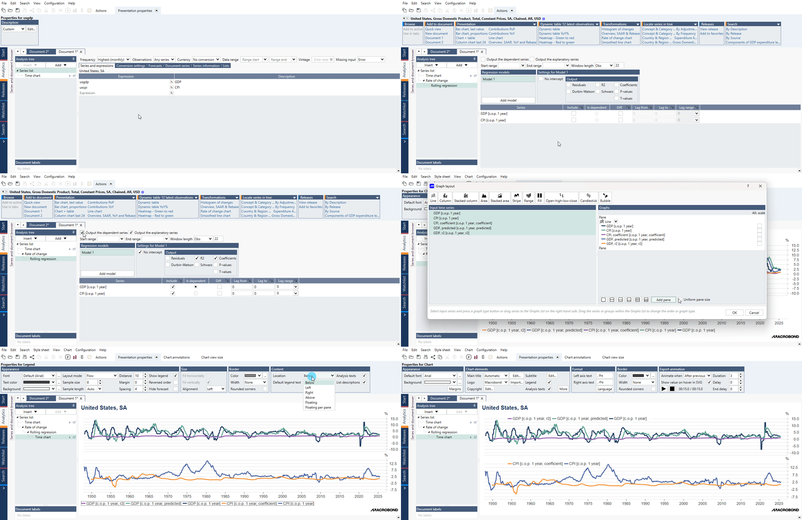
Example of general use of Rolling regression analysis additionally showing R2 and coefficient on chart:

The Rolling regression analysis implements a linear multivariate rolling window regression model. Just like ordinary regression, the analysis aims to model the relationship between a dependent series and one or more explanatory series. The difference is that in Rolling regression you define a window of a certain size that will be kept constant through the calculation. The analysis preforms a regression on the observations contained in the window, then the window is moved one observation forward in time and process is repeated. Thus, many regressions will be performed as the window moves forward.
Estimation model
For more in-depth information regarding the estimation model see Regression analysis.
Working with Rolling regression analysis
Settings
Regression models
You can define one or more regression models. Each model has separate settings. When a new model is created, the settings of the current model are duplicated. Models can be renamed and deleted.
Output dependent series
Select this option to include the dependent series in the output.
Output explanatory series
Select this option to include the explanatory series in the output.
Date range
Specify the limits of the date range and window length. The default range will be the largest range where there is data for all the series.
No intercept
When this option is selected, the constant α is omitted from the model and it will be defined as:
Residuals
When this option is selected a series containing the residuals will be included in the output.
Durbin-Watson
The Durbin-Watson is a test statistic used to detect the presence of autocorrelation in the residuals. The value is in the range 0-4. A value close to 2 means that there is little auto correlation. Values from 0 to less than 2 point to positive autocorrelation and values from 2 to 4 means negative autocorrelation. The result from this test is not useful if any dependent series is included with several lags or if no intercept is included in the model.
For more information about this see Investopedia.
Schwarz
The Schwarz information criterion takes overfitting into account and estimates the efficiency of the model in terms of predicting the data. The criterion yields a positive value, where a lower value is considered better when comparing different models based on the same data.
R2
The R2 value compares the variance of the estimation with the total variance. The better the result fits the data compared to a simple average, the closer this value is to 1.
Coefficient
The estimated parameters.
P-values
The p-value is the probability of obtaining a value of t that is at least as extreme as the one that was actually observed if the true value of the coefficient is zero.
T-values
The t-value measures the size of the difference relative to the variation in your sample data.
Series settings
Include
Select if you want to include this series in the model.
Is dependent
Select which series is the dependent series. This must be specified.
Diff
By selecting Diff, the first order differences of the series will be calculated. The result will then be converted back to levels. First order of differences means that the series is transformed to 'Change over value (one observation)' while expressing the result in levels. If you tick that option, the result will output the coefficients for intercept and diff(x1) rather than intercept and x1.
This setting does not affect the model itself. It only influences the step after the calculation of the model when the levels are calculated from the differences.
Lag to/from and Lag range
Here you specify the lags you would like to include for a specific series. When lagging a series, the values are delayed in time and the series stretches further into the future.
If you for example set “Lag from” to 0 and 'Lag to' to 2 three series will be included, one series with no lag, one with a lag of 1 and one series with 2 lags. This will automatically change the lag range to '0 to 2'. You may specify the desired lags using 'Lag to/from' or 'Lag range', the result will be the same. If you set Lag range to a single digit or set 'Lag to' and 'Lag from' to the same value, a single lagged series will be included.
When lags are specified for the dependent series, the lagged series will be used as explanatory series in the model. The dependent series will always be without lag.
How to create simple rolling regression model?
- Check box for 'Output the dependent series' or 'Output the explanatory series'.
- Select window length.
- Select Output indicators (they will appear on chart).
- Check 'Include' for at least two series and mark one as 'Is dependent'.
- Add Time chart.
Common errors
Degree of freedom is too low
You cannot fit the regression coefficients if there are no degrees of freedom. The degrees of freedom are the number of observations - number of parameters that we are estimating. The number of estimated parameters includes the intercept.
The number of observations must thus be larger than the number of independent (explanatory) series.
Forecast
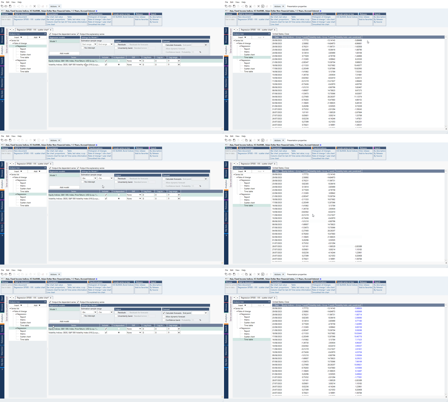
It is not possible to calculate forecast in Rolling regression analysis. In some way such functionality at some point would base forecast on itself because it keeps rolling.
As a workaround, we recommend using simple Regression analysis. In 'Estimation sample range' type in parameter '-window_length' (i.e.; -5m and -2m; -50 and -10). Thanks to that you will set last non-forecasted value in the desired point in time. When you enable 'Calculate forecast' box this will calculate the forecast based on the regression of the narrowed earlier number of observations of these two series.
Report
The fact that a rolling window is utilized has implications for the output. When using Regression analysis, a report is generated. In Rolling regression, no such report will be available. This is because, as explained in the overview, a rolling regression constitutes of many regressions, all of which will yield individual statistics. The output of statistics, information criteria and parameters will thus all be time series. You have many options regarding what information to include in the result.
How to output indicators?
Simply mark the indicator in the panel and it will be available as output.
Calculating regression with formulas
To calculate α and β use:
Intercept(series1, series2, window)
Slope(series1, series2, window)
where series1 is the dependent series and series2 is the explanatory series. If you get different values than from analysis check 'Estimation sample range' - it has to be calculated on identical time range. To avoid adding Cut() formula everywhere you can set data range on Series list.
Formulas above calculate the regression between two series, but if in Regression analysis are more series these won't be comparable models - you will get different outcomes.
Examples
In this example, we used the model presented for the Regression analysis, and created a new regression model which is generated on 5 years rolling window. For the output, we've included the residuals and the R2.
Here we calculate explanatory variable share.
Questions
- Why rolling regression's average residual is not zero?
- Why model's values are different than the ones coming from a same model but rolling?
Why rolling regression's average residual is not zero?
If you do a standard regression, the mean of the residuals is zero. With Rolling regression, it does one separate regressions at each point in time and thus residuals are not zero on average.
Why model's values are different than the ones coming from a same model but rolling?
The differences stems from different time ranges being taken into calculation because of:
- Mon-Sun daily series vs Mon-Fri daily series
- what Macrobond takes into account when calculating a sample range
To ensure that you are looking and comparing the exact same time periods use one of the below methods:
- change frequency in the document to Daily (not Daily (highest) or Daily (lowest)) and set Observations to Monday-Friday
- change the window size in Rolling regression from, for example 'X months', to number of observations in Regression i.e., '402'.
The first method will give closely similar results but still not 100% same due to the way Macrobond sets Start range i.e., '-18m' is not strictly '18m', but '18m' counting from the previous observation so, effectively '18 months +1'. In which case, you may want to set the Window length to a number of observations instead.
The latter approach will output the same values in both Regression and Rolling regression.
