Overview
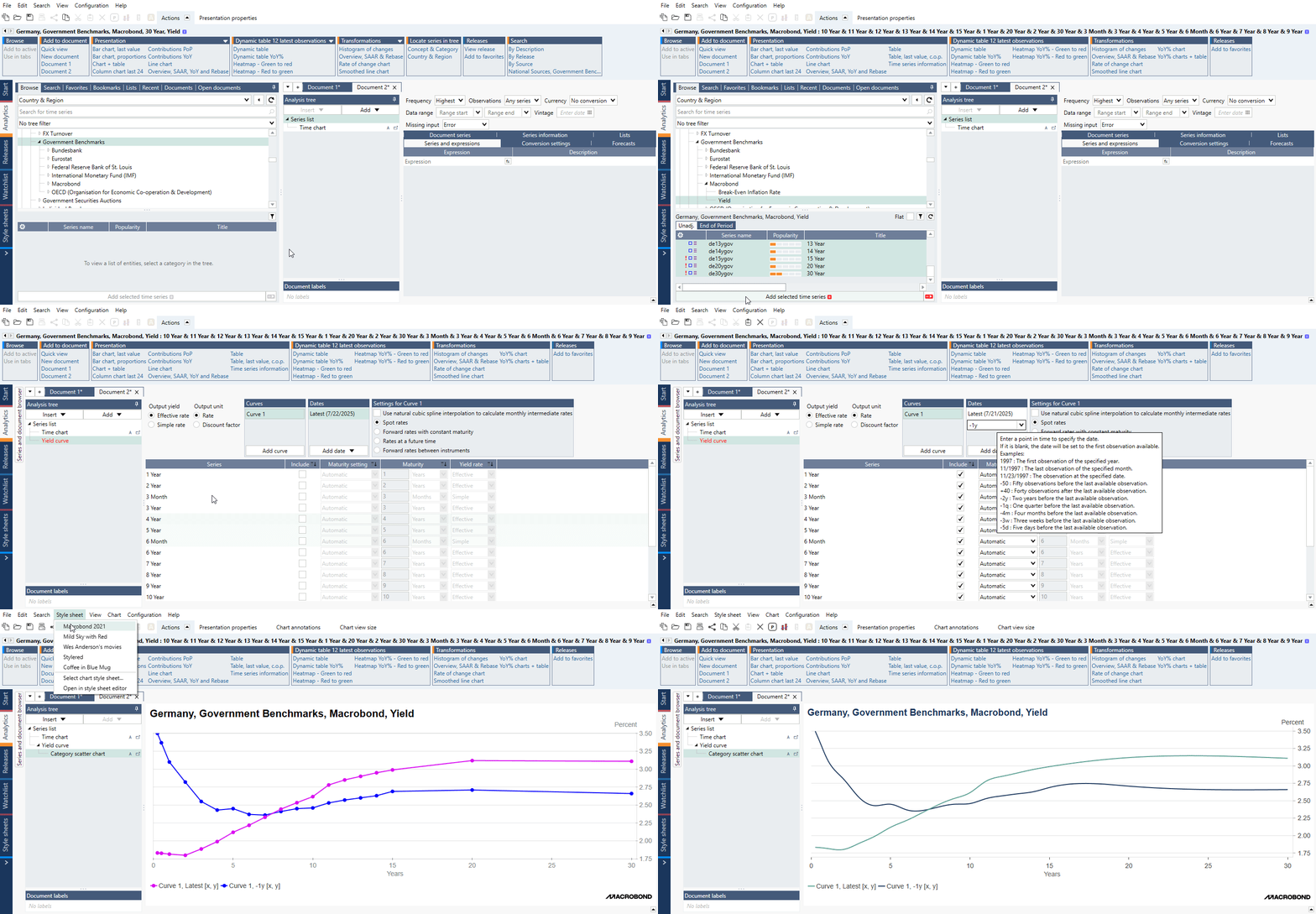
Example of general use of Yield curve analysis with curves for Latest and 1 year ago:
The Yield curve analysis lets you plot the yield across different contract lengths for similar debt contracts. This relationship is also known as the term structure of interest rates. You can calculate numerous curves at the same time with different dates, settings, and series. Combining several yield curves in a chart makes it easier to analyze trends over time and differences across regions.
Input & output
The input consists of a number of series with interest rates of different maturity lengths. If there is information in the database about maturity and the type of rate, effective or simple, the information will be filled in automatically. If that is not the case, you will have to define the parameters manually.
The analysis will produce two series for each yield curve. One series which contains the maturity lengths expressed as years and one series with the interest rate at the specified point in time for the corresponding maturity. This type of output is nicely visualized in a Category scatter chart.
Settings
Output yield
All input rates will be converted to either simple annual interest rate or effective annual interest rate. The relationship between the simple rate and the effective rate is:
where m is the maturity length expressed as the number of years.
Output unit
You can select to produce the discount factors instead of the interest rates. In this case the factors are calculated by one of these expressions depending on the type of rate:
Use natural cubic spline
When the option for natural cubic splines is selected, the curve will not only consist of points corresponding to the maturity lengths, but there will be a value at least every month. Intermediate values will be calculated by creating a natural cubic spline based on the rates. This will result in a smoother yield curve.
Spot rates
When 'Spot rates' is selected, the rate at each point in time will be used.
Forward rates with constant maturity
When 'Forward rates with constant maturity' is selected, you must also specify the length of the forward. The calculation of the forward rate will then be performed for each point on the curve by looking at the current rate and a future rate. If needed, the future rate is calculated by using a spline as described above.
Rates at a future time
With the option called 'Rates at a future time' forward rates that start at the point of the maturity length that you provide are calculated. This will give you a view of the yield curve at a future point in time relative to the observations.
Forward rates between instruments
The rate at each point is the rate of a forward from the corresponding instrument to the next. The length of the forward will thus be the difference in maturity of the current instrument and the next.
Day count convention
When specifying maturity lengths, the 30/360-day count convention is used. There are 360 days per year, 12 months per year and 7 days per week.
Please note that the Count parameter is a decimal number, and you can specify, for instance, 1.5 months.
Examples
In the example we calculate the yield curve for the US and Germany. For each country, both the current yield curve and the yield curve as of one year ago is calculated.
We have used Yield Curve on Future series and also calculated it manually with other analyses for comparison. Note that manual version keeps dates on x-axis. In this file we also used method which shows months on x-axis.
Rising number of 'Inverted' yield curves can signal recession. In this example we have calculate percent of inverted yield curves for United States.
Questions
- How to interpolate missing yield series?
- How to show percent of inverted yield curves?
- How to change x-axis to number of months instead of number of years?
- Why some series have Simple/Effective yield rate?
- Why value for 12m series is same under Simple and Effective rate method?
How to interpolate missing yield series?
In analysis you can enable to fill in intermediate observations using a natural cubic spline. Such a spline is smooth enough (here 'smooth' is used in a mathematical sense) to be arbitrage free and is therefore a good method to use for interpolation.
How to show percent of inverted yield curves?
You don't have to use Yield curve analysis to do this. See one of our examples above.
How to change x-axis to number of months instead of number of years?
There is a workaround which uses formulas and Cross section. See the solution in file Yield curve from Future series.
Why some series have Simple/Effective yield rate?
It is a standard practice that series under 1 year (i.e., those with no coupon paid) have Simple yield rate, series above 1 year (i.e., those with coupon paid) have Effective yield rate used.
Why value for 12m series is same under Simple and Effective rate method?
Series under 1 year have Simple yield rate while series above 1 year have Effective yield rate used. 12m securities are "on edge" and that's the reason why 12m is the same under both rate methods.
